
Key takeaways
- NDVI = (NIR − Red) / (NIR + Red). On Sentinel-2 that is (B8 − B4) / (B8 + B4); on Landsat 8 and 9 it is (B5 − B4) / (B5 + B4).
- Always calculate it from surface reflectance, not raw digital numbers, or values from different dates will not be comparable.
- Thresholds such as "above 0.6 is healthy" are local rules of thumb. Compare a field or forest with its own history before drawing conclusions.
- NDVI saturates over dense canopy and is sensitive to bright soil, so EVI, SAVI or NDRE are often better in those situations.
- A cloud-masked time series tells you far more than any single NDVI image.
Most people meet NDVI as a red-to-green map of farmland, and it is easy to treat that map as a direct picture of plant health. However, it is more useful, and more honest, to think of NDVI as a measurement of how much red light the surface absorbs compared with how much near-infrared light it reflects. In fact, healthy leaves happen to do both very strongly, which is why the index works. Therefore, knowing that one fact explains almost everything about where NDVI is reliable and where it can mislead you.
This guide covers how the index is calculated from Sentinel-2 and Landsat, how to read the values, the main applications, a practical workflow for building time series, and the limitations we check for on every project before an NDVI result goes to a client.
How NDVI works
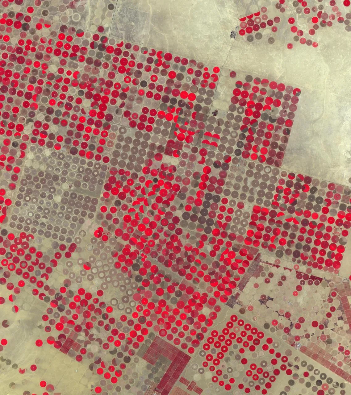
Chlorophyll absorbs red light (around 665 nm) to drive photosynthesis. The internal cell structure of a leaf, meanwhile, scatters near-infrared light (around 840 nm) very efficiently, so a healthy canopy can reflect 40 to 50 percent of incoming NIR while reflecting only a few percent of red. In contrast, bare soil reflects the two in similar amounts. Water absorbs NIR almost completely.
Then NDVI turns that contrast into a single number:
NDVI = (NIR − Red) / (NIR + Red)Moreover, dividing by the sum normalises the result to a range of −1 to +1 and cancels out part of the effect of illumination, slope and sun angle. That normalisation is the reason NDVI has been the standard vegetation index since researchers described it in the 1970s.
| Sensor | Red band | NIR band | Pixel size | Revisit |
| Sentinel-2 MSI | B4 | B8 (or B8A) | 10 m | About 5 days |
| Landsat 8 and 9 OLI | B4 | B5 | 30 m | 8 days combined |
| Landsat 5 and 7 TM/ETM+ | B3 | B4 | 30 m | 16 days each |
| MODIS | Band 1 | Band 2 | 250 m | Daily |
One detail catches many first-time users: the band numbers change between Landsat generations. A script written for Landsat 8 will produce nonsense on Landsat 7 data unless you update the band mapping.
Use surface reflectance, not digital numbers
Therefore, always calculate NDVI from atmospherically corrected surface reflectance: Sentinel-2 Level-2A, or Landsat Collection 2 Level-2. Haze adds brightness to the red band and lowers NDVI, so values calculated from top-of-atmosphere data drift from date to date even when nothing on the ground has changed. Landsat Collection 2 values also need their scale factor applied (multiply by 0.0000275 and add −0.2) before you calculate the ratio. In fact, skipping that step is one of the most common errors we see in inherited projects.
How to interpret NDVI values
| NDVI range | What it usually represents |
| Below 0 | Water, snow, cloud or deep shadow |
| 0 to 0.15 | Bare soil, sand, rock, roads and roofs |
| 0.15 to 0.35 | Sparse vegetation, dry grassland, crops just after emergence |
| 0.35 to 0.6 | Moderate cover: shrubland, pasture, crops in active growth |
| Above 0.6 | Dense green canopy: irrigated crops at peak, broadleaf forest |
Treat these ranges as a starting point. A wheat field at 0.45 in early March may be perfectly healthy, while a citrus orchard at 0.45 in midsummer may be stressed. Moreover, soil colour, row spacing, crop type, irrigation and sensor all shift the numbers. In practice, the most reliable reading comes from comparison: the same field against its own five-year average for that week, or one field against its neighbours planted with the same crop.
A worked example
Suppose a Sentinel-2 pixel over an irrigated alfalfa field has surface reflectance of 0.04 in B4 and 0.42 in B8. Therefore, NDVI is (0.42 − 0.04) / (0.42 + 0.04) = 0.83, a dense, actively growing canopy. Three weeks later, after a cut, the same pixel reads 0.09 in B4 and 0.24 in B8, giving 0.45. Nothing is wrong with the crop, because the drop simply reflects the harvest. Without the management calendar, however, an analyst could easily misreport that change as stress.
Applications of NDVI
Agriculture and crop monitoring
An NDVI curve through the season shows emergence, canopy development, peak and senescence. Agronomists use those curves to spot fields that green up late, plateau early or decline before harvest, then send scouts to check for water stress, pests, disease or nutrient problems. Within a field, for example, agronomists often use NDVI zones as a first layer for variable-rate fertiliser or irrigation planning.
Forest and land-cover mapping
NDVI is a standard input to land-cover classification because it separates vegetated from non-vegetated surfaces so cleanly. Seasonal NDVI statistics, such as the median, maximum and amplitude across a year, also help distinguish evergreen forest from deciduous forest and from cropland, which may look similar on a single date.
Drought and rangeland monitoring
Similarly, comparing current NDVI with the long-term average for the same period produces an anomaly map. Areas well below normal are an early warning of drought, often weeks before the impact appears in market or yield statistics. For example, famine early-warning systems and many national drought monitors use anomalies built from MODIS or Sentinel-2 NDVI.
Post-fire recovery
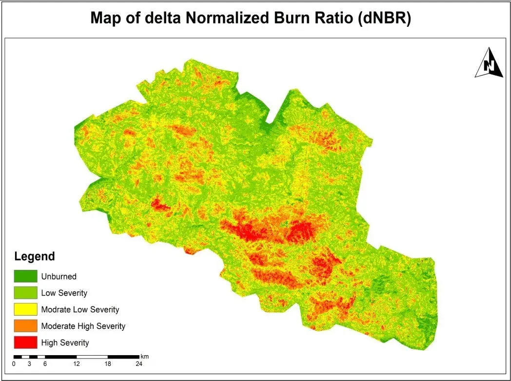
NDVI is not the best tool for measuring burn severity; NBR and dNBR do that job better because they use shortwave infrared. Once the severity map exists, though, NDVI is very effective for tracking how quickly vegetation returns in each severity class over the following seasons. That is the combination we use in burn assessments: dNBR to classify the damage, NDVI time series to follow recovery.
Calculating an NDVI time series
A single NDVI image is a snapshot. A time series shows behaviour, and behaviour is what most clients actually need to understand. This is the workflow we follow in Google Earth Engine, and the same logic applies in Python or QGIS.
- Define the area of interest and the period, usually several full seasons so the current year can be compared with a baseline.
- Load the surface reflectance collection (Sentinel-2 Level-2A or Landsat Collection 2 Level-2) filtered by area and date.
- Mask clouds and shadows for every image. For Sentinel-2 we use the Cloud Score+ product or the scene classification layer; for Landsat, the QA_PIXEL band.
- Calculate NDVI for each image and keep the acquisition date.
- Reduce to a regular interval, such as 10-day or monthly medians, to smooth out remaining noise.
- Extract statistics for each field or polygon and chart them against the multi-year average.
- Check unusual drops against high-resolution imagery or field notes before reporting them.
In Earth Engine, the core of the calculation is only a few lines:
var ndvi = s2.map(function(img) {
  return img.normalizedDifference(['B8', 'B4'])
            .rename('NDVI')
            .copyProperties(img, ['system:time_start']);
});
The time spent on cloud masking and validation is far greater than the time spent on the formula, and that is the right balance. A clean series with fewer dates is worth more than a dense series full of partly cloudy images.
Limitations of NDVI
- Saturation over dense canopy. Above roughly 0.8, NDVI changes very little even when leaf area keeps increasing. As a result, differences between a good and an excellent maize crop, or between two tropical forests, become hard to see. In contrast, EVI and the red-edge index NDRE hold up better in these conditions.
- Soil background. Where cover is sparse, bright or dark soil shifts the value. For this reason, SAVI adds a soil adjustment factor (usually L = 0.5) and is a better choice for arid rangeland and early-season crops.
- Atmosphere and cloud. Similarly, thin cloud and haze lower NDVI and can look like stress. Unmasked cloud shadow does the same. Masking is not optional.
- Sensor differences. Sentinel-2 and Landsat NDVI values are close but not identical. Mixing them in one series needs a harmonised product such as NASA's HLS or a cross-calibration step.
- Greenness is not yield or biomass. NDVI responds to green leaf area. A weedy field can look healthy, and a crop that has started to ripen will look stressed. Therefore, you still need field knowledge to interpret the signal.
Which index to use instead of, or alongside, NDVI
| Index | Best for | Bands (Sentinel-2) |
| EVI | Dense canopy, tropical forest | B8, B4, B2 |
| SAVI | Sparse vegetation, arid areas | B8, B4 |
| NDRE | Late-season crops, nitrogen status | B8A, B5 |
| NDMI | Canopy water content | B8A, B11 |
| NBR / dNBR | Burn severity | B8, B12 |
None of these replaces NDVI completely. On most projects we calculate NDVI for continuity and comparability, then add one or two indices chosen for the specific question.
Getting reliable results
In short, NDVI is simple to calculate and easy to misread. The projects that produce useful answers share the same habits: they use surface reflectance, mask clouds carefully, compare like with like over time, and check surprising results on the ground or in higher-resolution imagery before anyone acts on them. If you need NDVI monitoring for farms, rangeland or forest, our remote sensing and Google Earth Engine teams can set up a workflow that runs again each season without starting from scratch.
Frequently asked questions
What is a good NDVI value for crops?
For most field crops at peak growth, values between 0.6 and 0.85 are typical. Early in the season the same healthy field may read 0.2 to 0.3 because there is still a lot of bare soil between the plants. The useful question is not whether a value is "good" in general, but whether a field is tracking below its own previous seasons or below neighbouring fields of the same crop at the same stage.
Is NDVI free to calculate?
Yes. Sentinel-2 and Landsat imagery are free to download, and NDVI can be calculated in QGIS with the Raster Calculator, in ArcGIS Pro with the NDVI raster function, in Python with rasterio or xarray, or in Google Earth Engine. The only real cost is the time it takes to choose clean images and check the results.
What is the difference between NDVI and NBR?
NDVI uses red and near-infrared light and responds mainly to green leaf cover. The Normalized Burn Ratio uses near-infrared and shortwave infrared (Sentinel-2 B8 and B12, Landsat B5 and B7). Shortwave infrared rises sharply over charred ground and ash, so NBR, and the difference between pre-fire and post-fire NBR (dNBR), separates burn severity classes much more clearly than NDVI does.
Why does my NDVI map show negative values over a lake but also over some fields?
Water, snow and cloud reflect more red than near-infrared, so they produce negative values. If fields are negative, check for thin cloud, cloud shadow or a flooded paddy. It is also worth confirming that the bands were loaded in the right order, because swapping red and near-infrared flips the sign of the whole map.
Can NDVI estimate crop yield?
Not on its own. NDVI measures greenness, and greenness is only one part of yield. Integrated NDVI over the season often correlates well with yield for a given crop and region, but turning it into tonnes per hectare needs a model calibrated with harvest records from that area.
Related articles
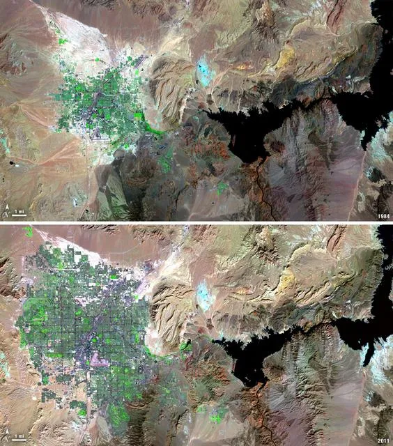
Satellite Change Detection: Methods, Accuracy and Real-World Applications
How satellite change detection works, which methods to use, where errors come from, and how indices such as NBR and dNBR turn imagery into measurable change.
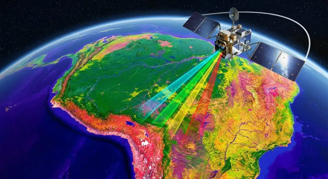
What Is Remote Sensing? How Satellites Observe the Earth and Why It Matters
A clear introduction to remote sensing and Earth observation: active and passive sensors, spectral bands, Landsat and Sentinel satellites, and real-world applications.