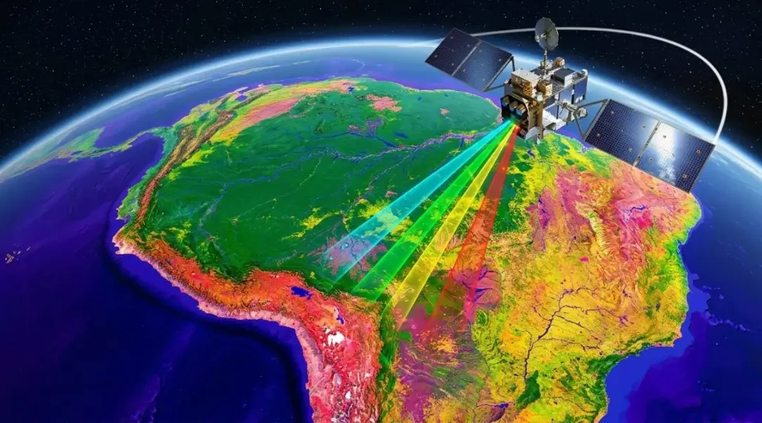
Satellite Change Detection: Methods, Accuracy and Real-World Applications

Satellite Change Detection: Methods, Accuracy and Real-World Applications

Satellite Change Detection: Methods, Accuracy and Real-World Applications

How satellite change detection works in practice: choosing image pairs, the main methods from index differencing to time-series analysis, a worked wildfire example with dNBR, and how to report change with an honest accuracy figure.

Remote SensingSpatial Nexus7 min read

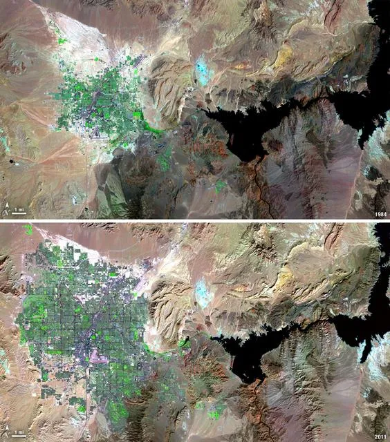
Landsat images of Las Vegas, Nevada, comparing urban expansion between two dates

Key takeaways

  • Most "change" in a careless analysis is not change at all. It is season, cloud, haze or misalignment between images.
  • Choose dates from the same season and, where possible, the same sensor, and work from surface reflectance.
  • Index differencing (NDVI, NDWI, dNBR) is fast and transparent; post-classification comparison tells you what changed into what.
  • Time-series methods such as LandTrendr and CCDC separate gradual trends from sudden events and are now practical in Google Earth Engine.
  • Report change as an area with a confidence interval, based on an independent accuracy sample, not as a raw pixel count.

Change detection is one of the most requested analyses in remote sensing, because the question behind it is simple: what is different now, and where? A ministry wants to know how much farmland housing has replaced. An insurer wants to see which fields flooded. A conservation project needs to prove that forest cover inside a reserve has held steady. In each case the answer comes from comparing images of the same place taken at different times.

The comparison itself is easy. Making sure the differences you find are real is where the work is. This guide explains how we choose imagery, the main methods and when each one fits, a worked wildfire example, the usual sources of error, and how to report results so they stand up to scrutiny.

What change detection actually measures

Every pixel in a satellite image records how much light the surface reflected in each band. If the surface changes, for example when someone clears a forest or a field floods, its spectral signature changes too. Change detection looks for pixels whose signature has shifted more than you would expect from normal variation.

The difficulty is that many things alter pixel values without any real change on the ground: the sun angle, haze, a slightly different sensor, soil moisture after rain, or simply the season. Therefore, a good analysis removes as much of that noise as possible before looking for change.
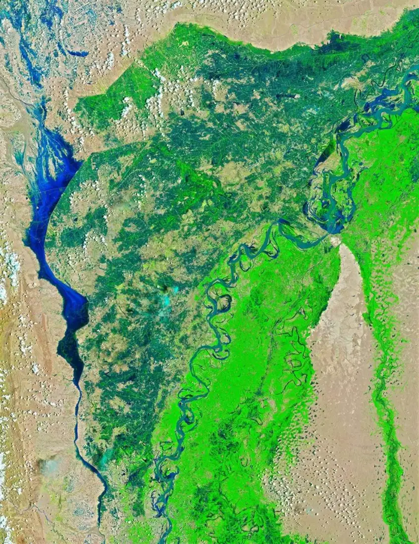
Landsat 8 false-colour image of the Indus River in Sindh before the 2022 floods
Before: Indus River, Sindh, 4 August 2022 (false colour; water appears dark blue).
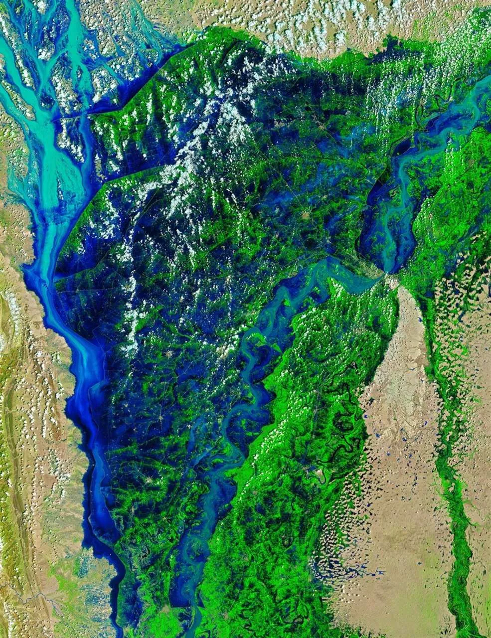
Landsat 9 false-colour image of the Indus River in Sindh during the 2022 floods
After: the same area on 28 August 2022, showing flood water spreading beyond the river channel.

Choosing the right images

Most problems in change detection start with the image pair. Before any processing, we check four things.

  • Season. Compare April with April, not April with October. Otherwise crops, deciduous trees and grassland will all appear to have changed.
  • Sensor. Use the same sensor family where possible. If you must mix Landsat and Sentinel-2, use a harmonised product such as NASA's HLS.
  • Processing level. Work from surface reflectance (Sentinel-2 Level-2A, Landsat Collection 2 Level-2) so that the same atmospheric correction applies on both dates.
  • Cloud and shadow. Mask them on both dates. An unmasked cloud on the first date and clear sky on the second will look exactly like new bare ground.

For events such as floods or fires, the "before" image should be as close to the event as possible while still being clear, and the "after" image should come once the event has peaked but before recovery or cleanup has started.

The main change detection methods

Image and index differencing

Calculate a spectral index on both dates and subtract one from the other. The analyst then flags pixels where the difference passes a threshold as changed. The choice of index follows the type of change:

Change of interestIndexWhy it works
Vegetation loss or gainNDVIResponds to green leaf cover
Surface water, floodsNDWI or MNDWIWater absorbs NIR and SWIR strongly
Burned area and severityNBR, giving dNBRSWIR rises sharply over char and ash
New built-up landNDBI, plus SWIR bandsRoofs and paving reflect SWIR

Differencing is fast, easy to explain and easy to repeat. Its weakness is the threshold: set it too low and you get false alarms, too high and you miss real change. We set thresholds by sampling known changed and unchanged areas rather than by eye.

Post-classification comparison

Classify each date independently into land-cover classes, then overlay the two maps. The output is a from–to matrix, for example 1,240 hectares of cropland converted to built-up land. This is the standard approach for land use and land cover change studies because the result is immediately meaningful to planners.

The catch is that errors multiply. If each classification is 88 percent accurate, the change map built from them will be noticeably less accurate than either, because a mistake on either date shows up as false change. Careful training data and the same class definitions on both dates are essential.

Time-series analysis

Instead of two dates, use every clear image over several years. Algorithms such as LandTrendr and CCDC fit a model to each pixel's history and flag the moment it breaks from its usual pattern. This separates a gradual decline, such as forest degradation, from a sudden event, such as clear-cutting, and it is much less affected by one unusual image.

Running these methods over large areas used to require serious computing resources. In Google Earth Engine they are now practical for a district or even a whole country.

Machine learning and deep learning

Alternatively, you can train supervised classifiers such as Random Forest directly on stacked before-and-after imagery to label change types. For very high-resolution imagery, deep learning models built on Siamese networks or U-Net architectures detect changes such as new buildings with impressive results. They need substantial labelled training data, so they make most sense for repeated monitoring of the same kind of change.

Worked example: measuring wildfire severity with dNBR

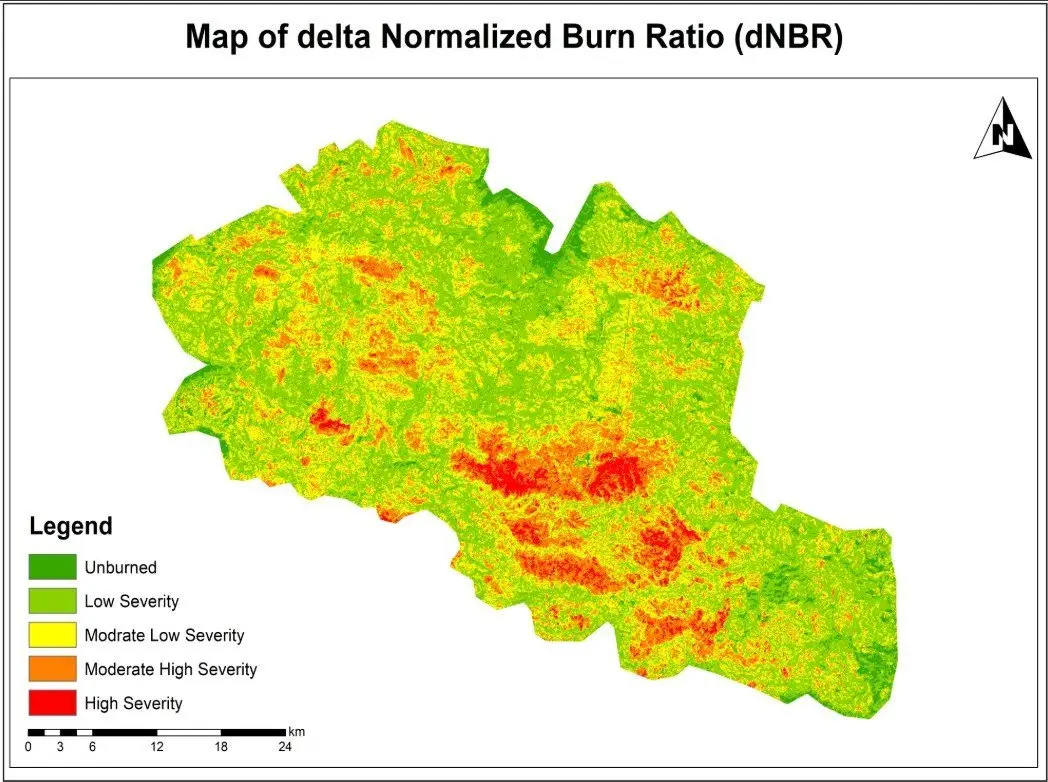
Our wildfire burn severity assessment is a good illustration of index differencing done carefully.

  1. We selected a clear Sentinel-2 image from before the fire and one from after it, as close to the same season as possible.
  2. We masked clouds and shadows on both dates.
  3. Next, we calculated the Normalized Burn Ratio for each date as (B8 − B12) / (B8 + B12).
  4. Then we calculated dNBR as pre-fire NBR minus post-fire NBR.
  5. The result was classified into severity classes using the widely used USGS ranges: below 0.1 unburned, 0.1 to 0.27 low, 0.27 to 0.44 moderate-low, 0.44 to 0.66 moderate-high, and above 0.66 high severity.
  6. Finally, we summarised burned area by severity class for reporting.

The map shows not just where the fire burned but how strongly it affected vegetation in each part of the area. That is what rehabilitation teams need, because high-severity zones are where erosion and slow regrowth are most likely.

Where change detection errors come from

  • Phenology. Seasonal greening and drying are the biggest source of false change in vegetated areas.
  • Residual cloud, haze and shadow. Even good cloud masks miss thin cirrus and some shadow edges.
  • Misregistration. If two images are offset by half a pixel, every field boundary and road edge appears as change. Sentinel-2 and Landsat products already align well, but drone and commercial imagery often need manual alignment.
  • Soil moisture and water levels. A wet field after rain looks very different from the same field dry.
  • Compounded classification errors in post-classification comparison.
  • Mixed pixels. At 30 m, a narrow new road or a small group of houses may only partly fill a pixel, so the analysis can miss it.

Measuring and reporting accuracy

A change map without an accuracy figure is an opinion. The approach we follow is the one that the remote sensing literature recommends and that national forest reporting uses:

  1. Draw a stratified random sample of points from each map class, including a separate stratum for change so rare changes are sampled well.
  2. Label each sample point independently using higher-resolution imagery or field data, without looking at the map.
  3. Build a confusion matrix and calculate overall, producer's and user's accuracy for each class.
  4. Use the sample to estimate the area of change with a 95 percent confidence interval, rather than simply counting mapped pixels.

The last step matters more than many people realise. Pixel counts inherit bias from the map's errors; sample-based area estimates correct for them. When a client needs to report deforestation or urban expansion to a funder or regulator, this is the figure that should be quoted.

Best practice checklist

  • Use same-season images from the same sensor family, in surface reflectance.
  • Mask clouds and shadows on every date and check the masks visually.
  • Choose the index or method that matches the type of change you are looking for.
  • Set thresholds from samples of known change, not by eye.
  • Validate with an independent, stratified sample and report area with uncertainty.
  • Document every step and parameter so the team can repeat the analysis next year.

Change detection rewards careful preparation more than clever algorithms. If you need change mapping for land cover, floods, fire or urban growth, our remote sensing and land use and land cover teams can design a workflow that gives you numbers you can defend. You can also see our land-cover change mapping project for a full example.

Frequently asked questions

Which satellite is best for change detection?

For most regional work, Sentinel-2 (10 m, roughly 5-day revisit) gives the best balance of detail and frequency. Landsat is the better choice when you need history, because its archive goes back to the 1980s at 30 m. Sentinel-1 radar is the right tool where cloud is persistent, such as monsoon floods. Commercial imagery below 1 m is worth the cost only when the features of interest, such as individual buildings, are smaller than a Sentinel-2 pixel.

How accurate is satellite change detection?

It depends on the type of change. Clear, large changes such as forest clearance, new reservoirs or severe burns often reach overall accuracies above 90 percent. Subtle changes such as forest degradation or crop rotation are much harder. The honest answer for any project is the accuracy measured against independent reference samples, reported with the class-by-class producer's and user's accuracy.

Can change detection be automated?

Yes, once you have tested the method for the area. We usually build the workflow in Google Earth Engine or Python so that every new image goes through exactly the same steps each month or season. Automation still needs a person reviewing flagged changes, at least until the false-alarm rate is known.

How often should we run change detection?

Match the frequency to how fast the change happens and how quickly you need to act. Flood and fire mapping is event-driven and often needed within days. Deforestation alerts are commonly weekly or monthly. Agencies usually report urban growth and land-cover change annually or every few years.

What is the difference between change detection and land-cover change mapping?

Change detection answers whether and where something changed. Land-cover change mapping goes further and labels the transition, for example cropland to built-up land. The second needs a classification for each date, which takes more effort but produces the from–to statistics planners usually ask for.

Need help applying this to your project?Talk to Spatial Nexus about remote sensing and earth observation for your area and data.

Discuss your project

  • change detection remote sensing
  • satellite change detection
  • dNBR burn severity
  • land cover change analysis
  • multi-temporal satellite imagery
Share this articleLinkedInEmail

Related articles

NDVI Explained: How Satellite Vegetation Indices Monitor Crops, Forests and Fire Recovery

NDVI Explained: How Satellite Vegetation Indices Monitor Crops, Forests and Fire Recovery

NDVI Explained: How Satellite Vegetation Indices Monitor Crops, Forests and Fire Recovery

How NDVI is calculated from Sentinel-2 and Landsat bands, what the values actually mean on the ground, where the index works well, where it misleads, and the workflow we use to build reliable NDVI time series.

Remote SensingSpatial Nexus7 min read

Burn severity map from the Normalized Burn Ratio with a five-class legend

Key takeaways

  • NDVI = (NIR − Red) / (NIR + Red). On Sentinel-2 that is (B8 − B4) / (B8 + B4); on Landsat 8 and 9 it is (B5 − B4) / (B5 + B4).
  • Always calculate it from surface reflectance, not raw digital numbers, or values from different dates will not be comparable.
  • Thresholds such as "above 0.6 is healthy" are local rules of thumb. Compare a field or forest with its own history before drawing conclusions.
  • NDVI saturates over dense canopy and is sensitive to bright soil, so EVI, SAVI or NDRE are often better in those situations.
  • A cloud-masked time series tells you far more than any single NDVI image.

Most people meet NDVI as a red-to-green map of farmland, and it is easy to treat that map as a direct picture of plant health. However, it is more useful, and more honest, to think of NDVI as a measurement of how much red light the surface absorbs compared with how much near-infrared light it reflects. In fact, healthy leaves happen to do both very strongly, which is why the index works. Therefore, knowing that one fact explains almost everything about where NDVI is reliable and where it can mislead you.

This guide covers how the index is calculated from Sentinel-2 and Landsat, how to read the values, the main applications, a practical workflow for building time series, and the limitations we check for on every project before an NDVI result goes to a client.

How NDVI works

Chlorophyll absorbs red light (around 665 nm) to drive photosynthesis. The internal cell structure of a leaf, meanwhile, scatters near-infrared light (around 840 nm) very efficiently, so a healthy canopy can reflect 40 to 50 percent of incoming NIR while reflecting only a few percent of red. In contrast, bare soil reflects the two in similar amounts. Water absorbs NIR almost completely.

Then NDVI turns that contrast into a single number:

NDVI = (NIR − Red) / (NIR + Red)

Moreover, dividing by the sum normalises the result to a range of −1 to +1 and cancels out part of the effect of illumination, slope and sun angle. That normalisation is the reason NDVI has been the standard vegetation index since researchers described it in the 1970s.

SensorRed bandNIR bandPixel sizeRevisit
Sentinel-2 MSIB4B8 (or B8A)10 mAbout 5 days
Landsat 8 and 9 OLIB4B530 m8 days combined
Landsat 5 and 7 TM/ETM+B3B430 m16 days each
MODISBand 1Band 2250 mDaily

One detail catches many first-time users: the band numbers change between Landsat generations. A script written for Landsat 8 will produce nonsense on Landsat 7 data unless you update the band mapping.

False-colour satellite image of centre-pivot irrigation in Al Jowf, Saudi Arabia, with healthy vegetation in red
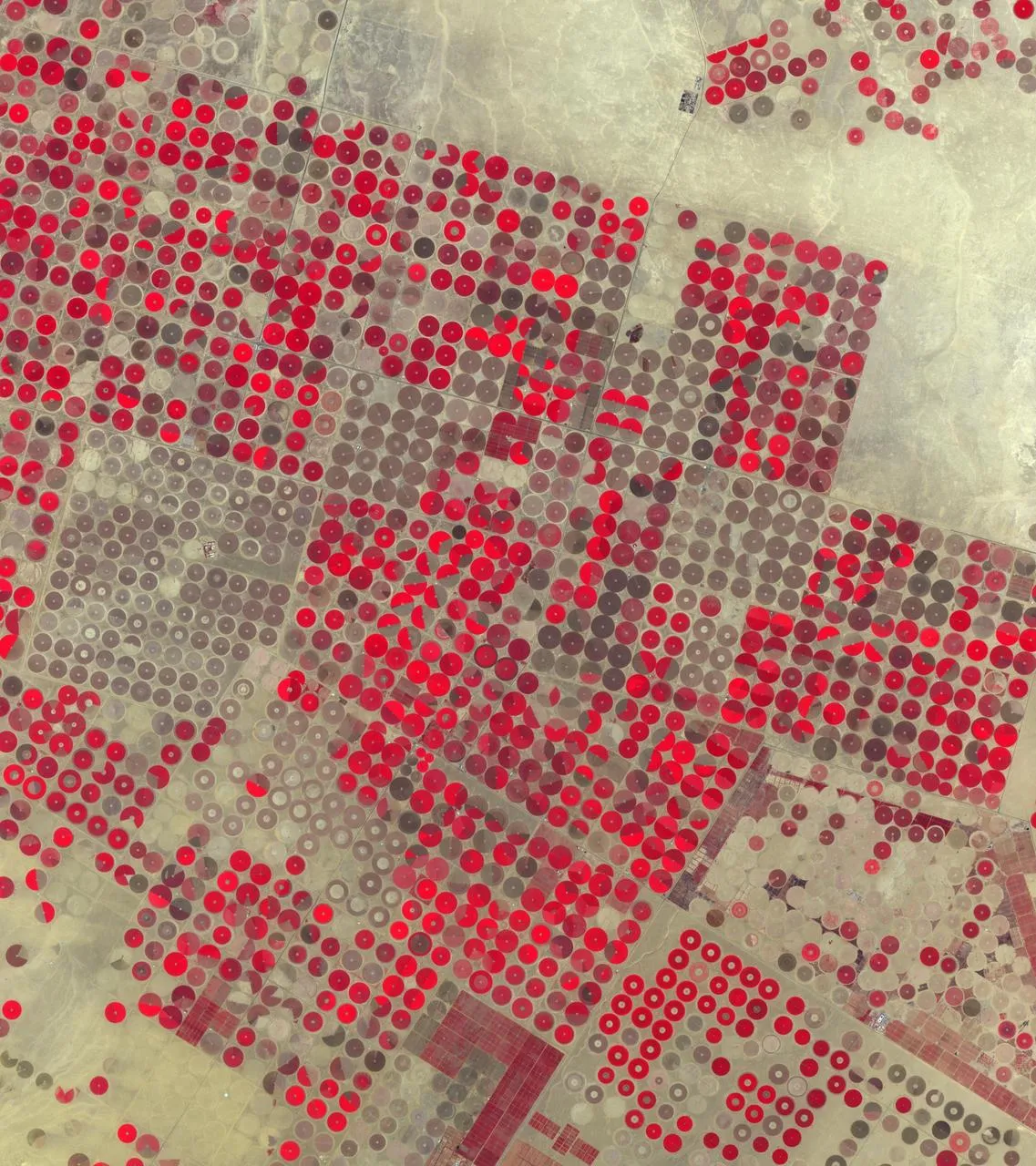
Centre-pivot fields in Al Jowf, Saudi Arabia, in false colour. Healthy vegetation appears red, the same signal NDVI measures.

Use surface reflectance, not digital numbers

Therefore, always calculate NDVI from atmospherically corrected surface reflectance: Sentinel-2 Level-2A, or Landsat Collection 2 Level-2. Haze adds brightness to the red band and lowers NDVI, so values calculated from top-of-atmosphere data drift from date to date even when nothing on the ground has changed. Landsat Collection 2 values also need their scale factor applied (multiply by 0.0000275 and add −0.2) before you calculate the ratio. In fact, skipping that step is one of the most common errors we see in inherited projects.

How to interpret NDVI values

NDVI rangeWhat it usually represents
Below 0Water, snow, cloud or deep shadow
0 to 0.15Bare soil, sand, rock, roads and roofs
0.15 to 0.35Sparse vegetation, dry grassland, crops just after emergence
0.35 to 0.6Moderate cover: shrubland, pasture, crops in active growth
Above 0.6Dense green canopy: irrigated crops at peak, broadleaf forest

Treat these ranges as a starting point. A wheat field at 0.45 in early March may be perfectly healthy, while a citrus orchard at 0.45 in midsummer may be stressed. Moreover, soil colour, row spacing, crop type, irrigation and sensor all shift the numbers. In practice, the most reliable reading comes from comparison: the same field against its own five-year average for that week, or one field against its neighbours planted with the same crop.

A worked example

Suppose a Sentinel-2 pixel over an irrigated alfalfa field has surface reflectance of 0.04 in B4 and 0.42 in B8. Therefore, NDVI is (0.42 − 0.04) / (0.42 + 0.04) = 0.83, a dense, actively growing canopy. Three weeks later, after a cut, the same pixel reads 0.09 in B4 and 0.24 in B8, giving 0.45. Nothing is wrong with the crop, because the drop simply reflects the harvest. Without the management calendar, however, an analyst could easily misreport that change as stress.

Applications of NDVI

Agriculture and crop monitoring

An NDVI curve through the season shows emergence, canopy development, peak and senescence. Agronomists use those curves to spot fields that green up late, plateau early or decline before harvest, then send scouts to check for water stress, pests, disease or nutrient problems. Within a field, for example, agronomists often use NDVI zones as a first layer for variable-rate fertiliser or irrigation planning.

Forest and land-cover mapping

NDVI is a standard input to land-cover classification because it separates vegetated from non-vegetated surfaces so cleanly. Seasonal NDVI statistics, such as the median, maximum and amplitude across a year, also help distinguish evergreen forest from deciduous forest and from cropland, which may look similar on a single date.

Drought and rangeland monitoring

Similarly, comparing current NDVI with the long-term average for the same period produces an anomaly map. Areas well below normal are an early warning of drought, often weeks before the impact appears in market or yield statistics. For example, famine early-warning systems and many national drought monitors use anomalies built from MODIS or Sentinel-2 NDVI.

Post-fire recovery

NDVI is not the best tool for measuring burn severity; NBR and dNBR do that job better because they use shortwave infrared. Once the severity map exists, though, NDVI is very effective for tracking how quickly vegetation returns in each severity class over the following seasons. That is the combination we use in burn assessments: dNBR to classify the damage, NDVI time series to follow recovery.

Calculating an NDVI time series

A single NDVI image is a snapshot. A time series shows behaviour, and behaviour is what most clients actually need to understand. This is the workflow we follow in Google Earth Engine, and the same logic applies in Python or QGIS.

  1. Define the area of interest and the period, usually several full seasons so the current year can be compared with a baseline.
  2. Load the surface reflectance collection (Sentinel-2 Level-2A or Landsat Collection 2 Level-2) filtered by area and date.
  3. Mask clouds and shadows for every image. For Sentinel-2 we use the Cloud Score+ product or the scene classification layer; for Landsat, the QA_PIXEL band.
  4. Calculate NDVI for each image and keep the acquisition date.
  5. Reduce to a regular interval, such as 10-day or monthly medians, to smooth out remaining noise.
  6. Extract statistics for each field or polygon and chart them against the multi-year average.
  7. Check unusual drops against high-resolution imagery or field notes before reporting them.

In Earth Engine, the core of the calculation is only a few lines:

var ndvi = s2.map(function(img) {
  return img.normalizedDifference(['B8', 'B4'])
            .rename('NDVI')
            .copyProperties(img, ['system:time_start']);
});

The time spent on cloud masking and validation is far greater than the time spent on the formula, and that is the right balance. A clean series with fewer dates is worth more than a dense series full of partly cloudy images.

Limitations of NDVI

  • Saturation over dense canopy. Above roughly 0.8, NDVI changes very little even when leaf area keeps increasing. As a result, differences between a good and an excellent maize crop, or between two tropical forests, become hard to see. In contrast, EVI and the red-edge index NDRE hold up better in these conditions.
  • Soil background. Where cover is sparse, bright or dark soil shifts the value. For this reason, SAVI adds a soil adjustment factor (usually L = 0.5) and is a better choice for arid rangeland and early-season crops.
  • Atmosphere and cloud. Similarly, thin cloud and haze lower NDVI and can look like stress. Unmasked cloud shadow does the same. Masking is not optional.
  • Sensor differences. Sentinel-2 and Landsat NDVI values are close but not identical. Mixing them in one series needs a harmonised product such as NASA's HLS or a cross-calibration step.
  • Greenness is not yield or biomass. NDVI responds to green leaf area. A weedy field can look healthy, and a crop that has started to ripen will look stressed. Therefore, you still need field knowledge to interpret the signal.

Which index to use instead of, or alongside, NDVI

IndexBest forBands (Sentinel-2)
EVIDense canopy, tropical forestB8, B4, B2
SAVISparse vegetation, arid areasB8, B4
NDRELate-season crops, nitrogen statusB8A, B5
NDMICanopy water contentB8A, B11
NBR / dNBRBurn severityB8, B12

None of these replaces NDVI completely. On most projects we calculate NDVI for continuity and comparability, then add one or two indices chosen for the specific question.

Getting reliable results

In short, NDVI is simple to calculate and easy to misread. The projects that produce useful answers share the same habits: they use surface reflectance, mask clouds carefully, compare like with like over time, and check surprising results on the ground or in higher-resolution imagery before anyone acts on them. If you need NDVI monitoring for farms, rangeland or forest, our remote sensing and Google Earth Engine teams can set up a workflow that runs again each season without starting from scratch.

Frequently asked questions

What is a good NDVI value for crops?

For most field crops at peak growth, values between 0.6 and 0.85 are typical. Early in the season the same healthy field may read 0.2 to 0.3 because there is still a lot of bare soil between the plants. The useful question is not whether a value is "good" in general, but whether a field is tracking below its own previous seasons or below neighbouring fields of the same crop at the same stage.

Is NDVI free to calculate?

Yes. Sentinel-2 and Landsat imagery are free to download, and NDVI can be calculated in QGIS with the Raster Calculator, in ArcGIS Pro with the NDVI raster function, in Python with rasterio or xarray, or in Google Earth Engine. The only real cost is the time it takes to choose clean images and check the results.

What is the difference between NDVI and NBR?

NDVI uses red and near-infrared light and responds mainly to green leaf cover. The Normalized Burn Ratio uses near-infrared and shortwave infrared (Sentinel-2 B8 and B12, Landsat B5 and B7). Shortwave infrared rises sharply over charred ground and ash, so NBR, and the difference between pre-fire and post-fire NBR (dNBR), separates burn severity classes much more clearly than NDVI does.

Why does my NDVI map show negative values over a lake but also over some fields?

Water, snow and cloud reflect more red than near-infrared, so they produce negative values. If fields are negative, check for thin cloud, cloud shadow or a flooded paddy. It is also worth confirming that the bands were loaded in the right order, because swapping red and near-infrared flips the sign of the whole map.

Can NDVI estimate crop yield?

Not on its own. NDVI measures greenness, and greenness is only one part of yield. Integrated NDVI over the season often correlates well with yield for a given crop and region, but turning it into tonnes per hectare needs a model calibrated with harvest records from that area.

Need help applying this to your project?Talk to Spatial Nexus about remote sensing and earth observation for your area and data.

Discuss your project

  • NDVI
  • normalized difference vegetation index
  • vegetation monitoring satellite
  • NDVI Google Earth Engine
  • crop health remote sensing
Share this articleLinkedInEmail

Related articles

What Is Remote Sensing? How Satellites Observe the Earth and Why It Matters

What Is Remote Sensing? How Satellites Observe the Earth and Why It Matters

What Is Remote Sensing? How Satellites Observe the Earth and Why It Matters

A clear introduction to remote sensing and Earth observation: how sensors measure reflected and emitted energy, passive and active systems, spectral bands and resolution, the Landsat and Sentinel missions, how raw images become analysis-ready data, and where it is used.

Remote SensingSpatial Nexus22 April 20266 min read

What-is-Remote-Sensing

Key takeaways

  • Remote sensing measures energy reflected or emitted by the Earth's surface, without physical contact.
  • Passive optical sensors need daylight and clear skies, whereas active radar works day and night and through cloud.
  • Each surface has a spectral signature. Comparing bands, for example red and near-infrared, reveals what the eye cannot see.
  • However, spatial, spectral, temporal and radiometric resolution always involve trade-offs. Therefore, choose the sensor for the question, not the sharpest image.
  • Moreover, Landsat and Sentinel provide free, calibrated imagery that covers most monitoring needs.

Every weather forecast, every flood map on the evening news and most modern crop monitoring systems depend on remote sensing. In fact, the term simply means gathering information about something without touching it. In Earth observation, for example, that something is the planet's surface and atmosphere, and the tools are sensors on satellites, aircraft and drones that record the energy coming from the ground.

This guide explains how remote sensing works, the types of sensors, what resolution really means, the missions that supply most of the world's free imagery, how raw images are turned into usable data, and the applications where it makes the biggest difference.

What is remote sensing?

To begin with, the Sun emits energy across the electromagnetic spectrum. When that energy reaches the Earth, surfaces absorb part of it, transmit part and reflect the rest. The surface also emits its own thermal energy. However, different materials do this in different ways at different wavelengths, which gives each one a characteristic pattern called a spectral signature.

  • Healthy vegetation absorbs red and blue light for photosynthesis and strongly reflects near-infrared.
  • Water absorbs most near-infrared and shortwave infrared, so it appears very dark in those bands.
  • Bare soil reflects gradually more as wavelength increases, with the level depending on moisture and mineral content.
  • Burned land has low near-infrared and high shortwave infrared reflectance.
  • Built-up surfaces are bright across many bands and especially in shortwave infrared.

Then a remote sensing instrument measures the energy reaching it in several wavelength bands. By comparing those measurements, analysts can tell vegetation from water, healthy crops from stressed ones, and fresh burns from bare soil.

How remote sensing works

Passive sensors

Passive sensors record energy that comes naturally from the scene: reflected sunlight or emitted heat. For example, the multispectral instruments on Landsat and Sentinel-2 are passive. They produce images that are easy to interpret, but they need daylight for reflected bands, and they cannot see through cloud. As a result, in monsoon regions this can mean weeks without a clear image.

Active sensors

In contrast, active sensors send their own signal and measure what returns.

  • Synthetic aperture radar (SAR), such as Sentinel-1, sends microwave pulses that pass through cloud and work at night. Radar responds to surface roughness, structure and moisture rather than colour. For example, calm water appears dark, which makes radar the main tool for flood mapping.
  • LiDAR sends laser pulses and times their return to measure heights very precisely. It produces detailed elevation models, building heights and forest canopy structure.

Spectral bands: seeing beyond visible light

In addition to visible light, optical satellites record several parts of the spectrum. The table below shows the main Sentinel-2 bands and what they are commonly used for.

BandWavelength (approx.)Pixel sizeCommon use
B2 Blue490 nm10 mTrue colour, water, atmosphere
B3 Green560 nm10 mTrue colour, water indices
B4 Red665 nm10 mVegetation (chlorophyll absorption)
B5 to B7 Red edge705 to 783 nm20 mCrop condition, nitrogen status
B8 Near-infrared842 nm10 mVegetation vigour, NDVI
B11 SWIR 11610 nm20 mMoisture, built-up areas, MNDWI
B12 SWIR 22190 nm20 mBurn severity (NBR), geology

Combining bands creates false-colour images and indices. Showing near-infrared as red, for example, makes healthy vegetation appear bright red. Indices such as NDVI for vegetation, MNDWI for water and NBR for burned areas turn these differences into numbers that can be mapped and compared over time.

The four kinds of resolution

ResolutionMeaningExample
SpatialGround size of one pixelSentinel-2: 10 m; Landsat: 30 m; commercial: 30 to 50 cm
SpectralNumber and width of bandsSentinel-2: 13 bands; hyperspectral sensors: hundreds
TemporalHow often the same place is imagedSentinel-2: about 5 days; MODIS: daily
RadiometricHow finely brightness is recordedLandsat 9: 14-bit; older Landsat: 8-bit

There is always a trade-off. However, sensors with very fine pixels usually cover smaller areas, revisit less often and cost more. For most regional monitoring, 10 to 30 m imagery with frequent revisits is more useful than occasional 50 cm images.

The satellites doing the work

Landsat

Operated by NASA and the U.S. Geological Survey, Landsat has imaged the Earth continuously since 1972. Landsat 8 and Landsat 9 now work together to provide 30 m multispectral imagery every 8 days, plus a 15 m panchromatic band and thermal bands. Also, the archive is free and consistently processed, which makes Landsat unmatched for change analysis over decades.

Sentinel

The European Union's Copernicus programme operates the Sentinel family, all with free and open data.

  • Sentinel-1: C-band radar for floods, ground movement, sea ice and crops, in any weather.
  • Sentinel-2: 13-band optical imagery at 10 to 60 m, with a revisit of about five days.
  • Sentinel-3: ocean colour, land and sea surface temperature at coarser resolution.
  • Sentinel-5P: atmospheric gases such as nitrogen dioxide and methane.

MODIS and VIIRS

In contrast, these sensors image the whole planet daily at 250 m to 1 km. Generally, analysts use them for vegetation anomalies, fire detection, snow cover and night-time lights.

Commercial satellites

Commercial constellations from companies such as Maxar, Airbus and Planet provide imagery down to about 30 cm, or daily coverage at 3 to 5 m. Consequently, they are the right choice for mapping individual buildings, small infrastructure and rapid change at site level.

From raw image to analysis-ready data

A satellite image straight from the sensor is a grid of numbers that still contains distortions. Before analysis, imagery goes through several steps, most of which the data providers now do for you.

  1. Radiometric calibration converts raw digital numbers into physical units of radiance or reflectance.
  2. Atmospheric correction removes the effect of haze and gases to give surface reflectance. Fortunately, the agencies already correct Sentinel-2 Level-2A and Landsat Collection 2 Level-2 products.
  3. Geometric correction aligns the image with a map coordinate system and corrects for terrain.
  4. Cloud and shadow masking removes contaminated pixels.
  5. Compositing combines several images, for example a monthly median, to fill gaps.

Working from analysis-ready products saves time and, more importantly, makes results from different dates comparable.

Remote sensing applications

Disaster response

Before-and-after imagery maps floods, landslides, earthquake damage and wildfire extent within hours or days. Our wildfire burn severity assessment used Sentinel-2 imagery with NBR and dNBR to classify damage from unburned to high severity.

Agriculture and food security

For example, vegetation indices track crop growth through the season, flag stress early and support yield estimates over whole regions. Our vegetation condition time series in Google Earth Engine is an example.

Climate and environment

Long satellite records measure changes in forests, glaciers, snow, coastlines, surface temperature and water bodies, and provide consistent indicators for national and international reporting.

Water resources

Imagery tracks reservoir levels, irrigation, wetlands and river course changes, and radar maps floods through cloud.

Urban planning and infrastructure

Similarly, imagery shows where cities are growing, maps impervious surfaces and urban heat, and provides current base maps for planning and asset management.

Forestry and conservation

Optical and radar data detect deforestation and degradation, and LiDAR measures canopy height and biomass.

Limitations to keep in mind

  • To begin with, cloud, smoke and darkness block optical imagery.
  • Pixels larger than the features of interest produce mixed signals.
  • Also, derived maps are models and contain errors, so you need to validate them.
  • Similarly, you still need ground data for training classifiers and checking results.

Remote sensing is at its best when it is paired with good ground knowledge and a clear question. If you need imagery analysis for monitoring, mapping or reporting, our remote sensing and Earth observation team can help you choose the right data and methods.

Frequently asked questions

What is the difference between remote sensing and GIS?

In short, remote sensing is the way you collect data: sensors on satellites, aircraft or drones measuring the surface from a distance. GIS, on the other hand, is the system that stores, analyses and maps spatial data. In practice they work together: remote sensing provides imagery and derived layers such as land cover or flood extent, and GIS combines them with roads, boundaries, population and other data to answer a question.

How accurate is satellite imagery?

It depends on what you mean by accurate. Positional accuracy for Sentinel-2 and Landsat is typically within about one pixel or better, so roughly 10 m and 30 m respectively. For example, commercial imagery can be accurate to a few metres. The accuracy of products derived from imagery, such as a land-cover map, depends on the method and should always be measured against reference data and reported.

Can anyone access satellite imagery?

Yes. Landsat imagery is free from the USGS, and Sentinel imagery is free from the Copernicus Data Space Ecosystem. Both are also available in Google Earth Engine and Microsoft's Planetary Computer. Very high-resolution commercial imagery from providers such as Maxar, Airbus and Planet is paid, though some programmes offer it for research and humanitarian use.

Is remote sensing only done by satellites?

No. Aircraft carry high-resolution cameras, LiDAR and hyperspectral sensors for detailed surveys. Meanwhile, surveyors widely use drones for site-scale mapping, crop scouting and construction monitoring. Ground-based instruments, such as spectroradiometers and terrestrial laser scanners, are also forms of remote sensing.

What resolution do I need?

Choose the coarsest resolution that still shows the features you care about, because finer imagery costs more, covers less and is harder to process. For instance, regional crop or drought monitoring works well at 10 to 30 m. However, mapping individual buildings or trees needs 1 m or better. Finally, daily monitoring of large areas may favour 250 m MODIS or 300 m Sentinel-3.

Need help applying this to your project?Talk to Spatial Nexus about remote sensing and earth observation for your area and data.

Discuss your project

  • remote sensing
  • satellite imagery
  • Earth observation
  • Landsat and Sentinel
  • remote sensing applications
Share this articleLinkedInEmail

Related articles