Wildfire Burn Severity Assessment Using NBR & dNBR (Remote Sensing Analysis)

Wildfire Burn Severity Assessment Using NBR & dNBR (Remote Sensing Analysis)

Wildfire Burn Severity Assessment Using NBR & dNBR (Remote Sensing Analysis)

Assessing wildfire burn severity and vegetation recovery using Sentinel-2 imagery and the Normalized Burn Ratio (NBR) and differenced NBR (dNBR).

About this project

Project overview

Monitoring wildfire impact is critical for environmental management, ecological recovery, and risk mitigation. In this project, Spatial Nexus conducted an advanced remote sensing analysis using Sentinel-2 satellite imagery to assess wildfire burn severity and post-fire vegetation recovery.

By leveraging Normalized Burn Ratio (NBR) and delta NBR (dNBR) techniques, we developed a data-driven framework to quantify damage and support rehabilitation planning and environmental decision-making.

  • burn severity mapping
  • dNBR remote sensing
  • Sentinel-2 wildfire analysis
  • Normalized Burn Ratio
  • post-fire vegetation recovery

Project at a glance

Client
Environmental and disaster management
Sector
Environment
Software
Sentinel-2 Satellite Imagery, GIS Platforms, Google Earth, Remote Sensing Techniques

THE CHALLENGE

What needed solving

  • Field surveys of large burned areas are slow, costly and sometimes unsafe.
  • Decision-makers needed to know not only where the fire burned but how severely.
  • Results had to support rehabilitation planning and long-term monitoring.

OBJECTIVES

What the project set out to do

  • Map burn extent and severity from satellite imagery.
  • Classify severity into standard classes.
  • Provide a basis for monitoring post-fire vegetation recovery.

Methodology

Our workflow, step by step

01

Image selection

Cloud-free Sentinel-2 scenes were selected before and after the fire.

02

NBR calculation

The Normalized Burn Ratio was calculated for each date from near-infrared and shortwave-infrared bands.

03

dNBR differencing

Post-fire NBR was subtracted from pre-fire NBR to measure change.

04

Severity classification

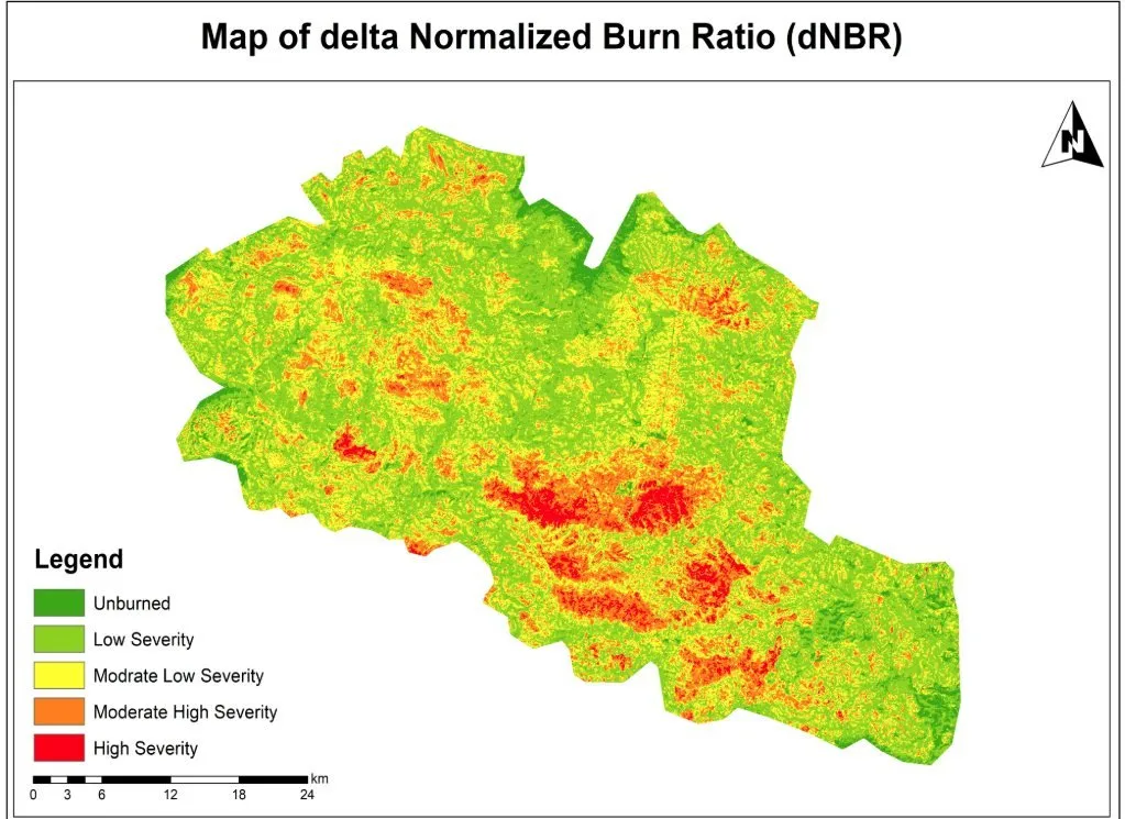
dNBR values were classified from unburned to high severity.

05

Validation and mapping

Results were checked visually against reference imagery and presented as a severity map.

Visual output

The map

Select the image to view it at full size.

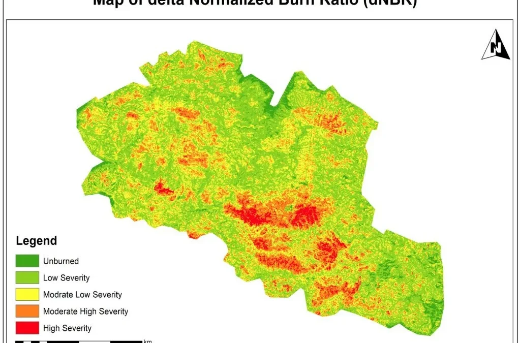
Wildfire Burn Severity Assessment Using NBR & dNBR (Remote Sensing Analysis), map output

Results

What the analysis delivered

  • A burn severity map showing unburned, low, moderate-low, moderate-high and high severity zones.
  • Clear identification of the most severely affected areas for priority action.
  • A baseline for monitoring vegetation recovery over time.

Key highlights

Why this project stands out

  • Sentinel-2 multispectral analysis
  • NBR and dNBR modelling
  • Five-class severity classification
  • Supports recovery monitoring

Data sources

Data used

  • Sentinel-2 pre-fire imagery
  • Sentinel-2 post-fire imagery
  • Google Earth reference imagery for validation

Tools and technologies

Software and methods

Sentinel-2 Satellite ImageryHigh-resolution Earth observation data
GIS PlatformsSpatial analysis and mapping
Google EarthVisualization and validation
Remote Sensing TechniquesNBR & dNBR modeling

Deliverables

What the client received

  • Burn severity map
  • NBR and dNBR rasters
  • Severity class statistics
  • Method note

WHY IT MATTERS

Satellite-based burn severity mapping enables rapid damage assessment, targeted restoration and long-term environmental monitoring as wildfires become more frequent.

FAQ

Questions about this project

What is dNBR?

The differenced Normalized Burn Ratio, calculated by subtracting post-fire NBR from pre-fire NBR. Higher values indicate more severe burning.

Why use Sentinel-2?

It provides free 10–20 m imagery with the near-infrared and shortwave-infrared bands needed for NBR, revisiting every few days.

Can recovery be monitored?

Yes. Repeating the analysis over later seasons shows how vegetation returns.

Planning a similar geospatial project?

Land-cover change mapping for a regional land-use plan

Land-cover change mapping for a regional land-use plan

Land-cover change mapping for a regional land-use plan

Classification of two satellite dates to map where vegetation, cropland and built-up land changed.

About this project

Project overview

Example workflow showing how Spatial Nexus approaches this type of analysis.

Classification of two satellite dates to map where vegetation, cropland and built-up land changed.

This page shows a typical Spatial Nexus workflow for this type of analysis.

  • land cover change mapping
  • LULC classification
  • Google Earth Engine land cover
  • remote sensing change detection
  • regional land use planning

Project at a glance

Sector
Remote Sensing
Software
Google Earth Engine, QGIS, Python, ERDAS IMAGINE, ENVI, ArcGIS Pro

THE CHALLENGE

What needed solving

  • Land-use plans need evidence of how land cover has changed.
  • Manual interpretation of large areas is slow and inconsistent.

OBJECTIVES

What the project set out to do

  • Classify land cover for two dates.
  • Quantify change between classes.
  • Report accuracy transparently.

Methodology

Our workflow, step by step

01

Pre-processing

Cloud masking and compositing for each date.

02

Classification

Supervised classification into agreed land-cover classes.

03

Accuracy assessment

Confusion matrix against independent reference points.

04

Change analysis

Cross-tabulation of classes between the two dates.

Visual output

The map

Select the image to view it at full size.

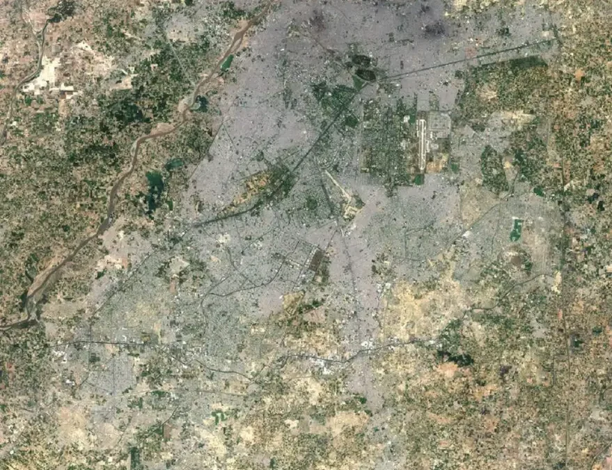
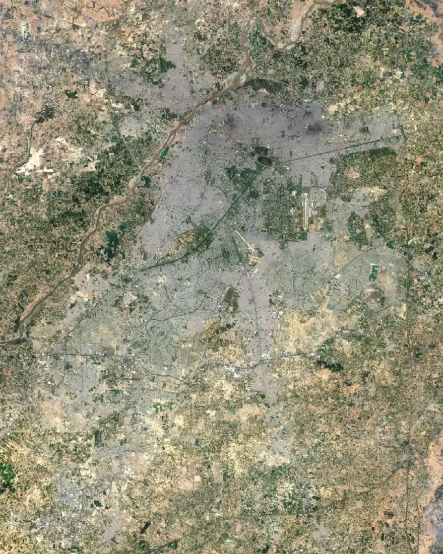
Landsat 8 natural-colour image of Lahore and the Ravi River, May 2024

Results

What the analysis delivered

  • Land-cover maps for each date.
  • A from–to change matrix with area statistics.
  • Accuracy assessment with confusion matrix.

Key highlights

Why this project stands out

  • Pre-processing
  • Classification
  • Accuracy assessment
  • Change analysis

Data sources

Data used

  • Landsat or Sentinel-2 imagery for two dates
  • Reference samples for training and validation

Tools and technologies

Software and methods

Google Earth Engine
QGIS
Python
ERDAS IMAGINE
ENVI
ArcGIS Pro

Deliverables

What the client received

  • Land-cover rasters and vectors
  • Area statistics and change matrix
  • Confusion matrix and accuracy figures
  • Map series

FAQ

Questions about this project

Which classes are mapped?

Classes are agreed with the client, typically water, vegetation, cropland, bare land and built-up areas.

How is accuracy measured?

With independent reference samples and a confusion matrix reporting overall and per-class accuracy.

Planning a similar geospatial project?

Vegetation condition time series in Earth Engine

Vegetation condition time series in Earth Engine

Vegetation condition time series in Earth Engine

A reproducible script tracking seasonal vegetation index trends across several years.

About this project

Project overview

Example workflow showing how Spatial Nexus approaches this type of analysis.

A reproducible script tracking seasonal vegetation index trends across several years.

This page shows a typical Spatial Nexus workflow for this type of analysis.

  • NDVI time series
  • Google Earth Engine vegetation monitoring
  • crop monitoring remote sensing
  • seasonal vegetation analysis
  • Earth Engine scripting

Project at a glance

Sector
Remote Sensing
Software
Google Earth Engine, Python, R

THE CHALLENGE

What needed solving

  • Single images cannot show seasonal or long-term vegetation trends.
  • Processing years of imagery locally is slow.

OBJECTIVES

What the project set out to do

  • Build a reproducible Earth Engine script.
  • Track seasonal NDVI over several years.

Methodology

Our workflow, step by step

01

Collection

Filter imagery by area, date and cloud cover.

02

Index

Calculate NDVI per image.

03

Compositing

Build seasonal composites.

04

Trend

Chart and map trends per zone.

Visual output

The map

Select the image to view it at full size.

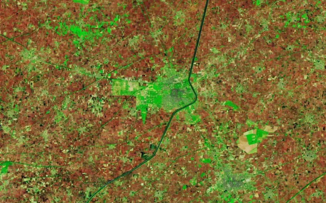
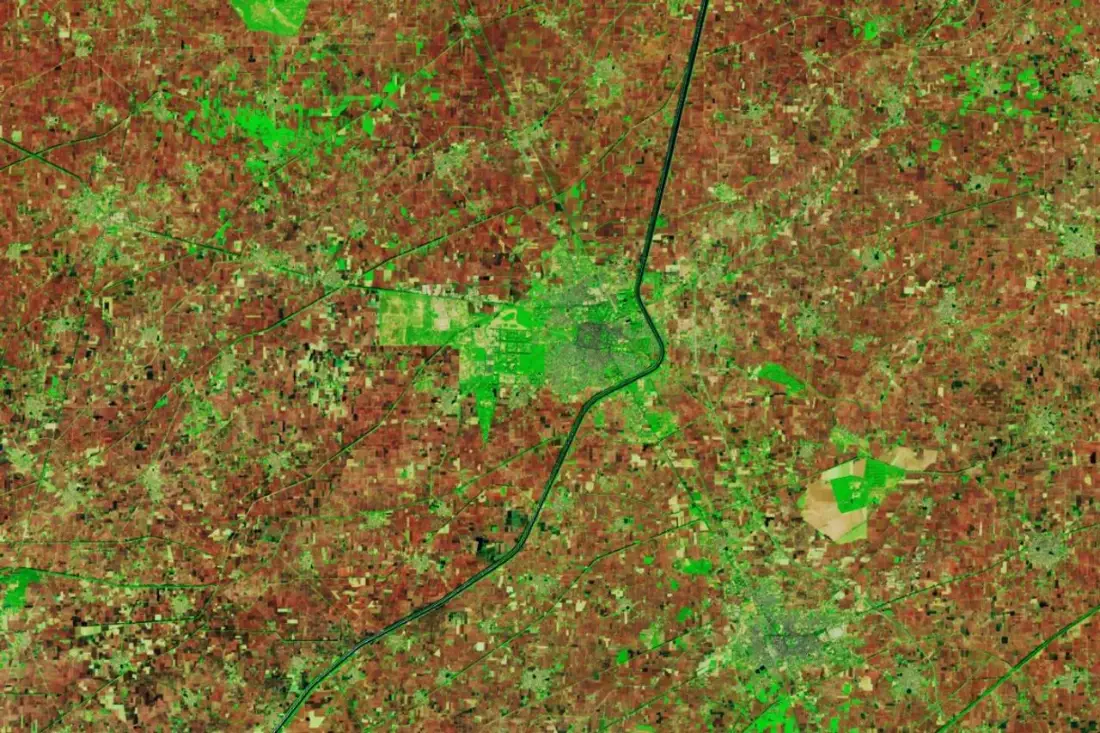
Landsat 9 false-colour image of farm fields near Faridkot, Punjab, with burned and vegetated fields

Results

What the analysis delivered

  • Seasonal NDVI composites and trend charts.
  • A script that updates as new imagery arrives.

Key highlights

Why this project stands out

  • Collection
  • Index
  • Compositing
  • Trend

Data sources

Data used

  • Sentinel-2 and Landsat archives
  • Area of interest boundary

Tools and technologies

Software and methods

Google Earth Engine
Python
R

Deliverables

What the client received

  • Documented Earth Engine scripts
  • Exported rasters and charts
  • Earth Engine app where useful
  • Method note

FAQ

Questions about this project

Why Google Earth Engine?

It hosts petabytes of satellite data and processes long time series in the cloud.

Can results be exported?

Yes. Rasters and charts can be exported for reports and GIS.

Planning a similar geospatial project?

Flood susceptibility mapping for a river catchment

Flood susceptibility mapping for a river catchment

Flood susceptibility mapping for a river catchment

Terrain, land cover, rainfall and soil factors combined to map relative flood susceptibility.

About this project

Project overview

Example workflow showing how Spatial Nexus approaches this type of analysis.

Terrain, land cover, rainfall and soil factors combined to map relative flood susceptibility.

This page shows a typical Spatial Nexus workflow for this type of analysis.

  • flood susceptibility mapping
  • flood risk GIS
  • remote sensing flood mapping
  • hydrological analysis
  • disaster risk reduction GIS

Project at a glance

Sector
Environment
Software
QGIS, Google Earth Engine, ArcGIS Pro, Global Mapper, ERDAS IMAGINE

THE CHALLENGE

What needed solving

  • Flood-prone areas must be identified before events occur.
  • Evidence is needed to prioritise mitigation.

OBJECTIVES

What the project set out to do

  • Combine terrain, drainage, rainfall and land cover.
  • Produce a flood susceptibility map.

Methodology

Our workflow, step by step

01

Factors

Derive slope, elevation, distance to drainage and land cover.

02

Weighting

Weight factors using an agreed method.

03

Model

Combine into a susceptibility index.

04

Validation

Compare with recorded flood extents where available.

Visual output

The map

Select the image to view it at full size.

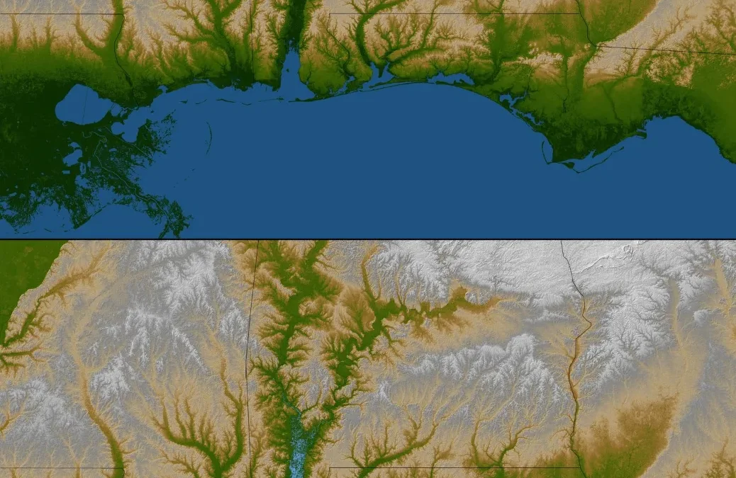
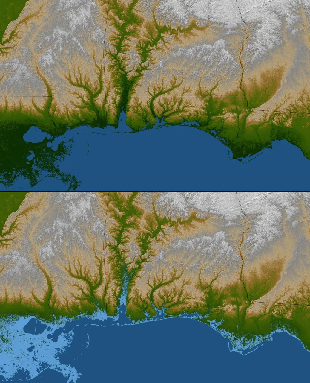
Gulf Coast shaded relief and colour-coded elevation highlighting low-lying land prone to flooding

Results

What the analysis delivered

  • Flood susceptibility classes from very low to very high.
  • Validation against observed flood extents.

Key highlights

Why this project stands out

  • Factors
  • Weighting
  • Model
  • Validation

Data sources

Data used

  • Elevation model and derived slope
  • Drainage network
  • Rainfall and land-cover data
  • Historical flood extents from satellite imagery

Tools and technologies

Software and methods

QGIS
Google Earth Engine
ArcGIS Pro
Global Mapper
ERDAS IMAGINE

Deliverables

What the client received

  • Hazard and susceptibility maps
  • Watershed and drainage layers
  • Indicator time series
  • Method and limitations note

FAQ

Questions about this project

What is flood susceptibility?

The relative likelihood that an area will flood, based on its physical characteristics.

How is it validated?

By comparing predicted zones with flood extents mapped from satellite imagery.

Planning a similar geospatial project?

Multi-Temporal Satellite Monitoring with Google Earth Engine

Multi-Temporal Satellite Monitoring with Google Earth Engine

Multi-Temporal Satellite Monitoring with Google Earth Engine

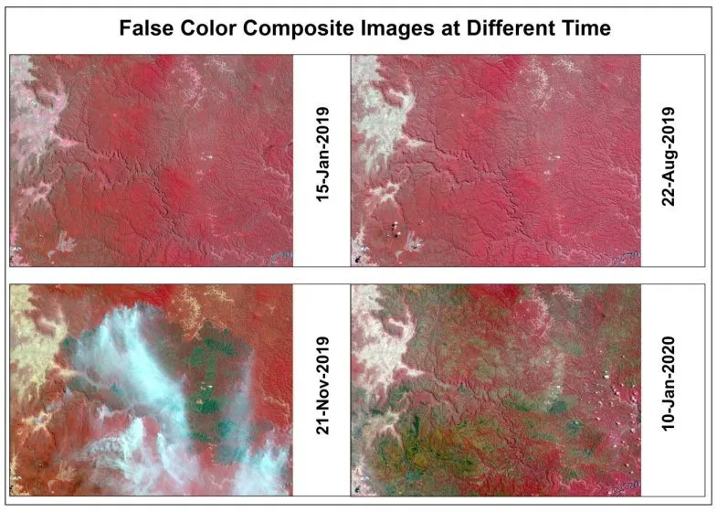
Using Google Earth Engine to compare true-colour and false-colour satellite composites across four dates and track seasonal and land-surface change.

About this project

Project overview

Using Google Earth Engine to compare true-colour and false-colour satellite composites across four dates and track seasonal and land-surface change.

  • Google Earth Engine
  • multi-temporal satellite imagery
  • false color composite
  • satellite time series analysis
  • Earth Engine remote sensing

Project at a glance

Client
Environmental monitoring
Sector
Environment
Software
Google Earth Engine, Sentinel-2 / Landsat, QGIS, Python, ENVI

THE CHALLENGE

What needed solving

  • Change between seasons is hard to see in single natural-colour images.
  • Downloading and processing many scenes locally is slow.
  • Cloud cover affected some dates.

OBJECTIVES

What the project set out to do

  • Build comparable composites for four dates.
  • Use false-colour band combinations to highlight vegetation and surface change.
  • Produce clear comparison panels for reporting.

Methodology

Our workflow, step by step

01

Filtering

Imagery was filtered in Earth Engine by area, date and cloud cover.

02

Cloud masking

Cloud and shadow were masked to keep composites clean.

03

Composites

True-colour and false-colour composites were built for each date.

04

Comparison layout

Composites were arranged as dated panels for side-by-side comparison.

Visual output

The map

Spatial Nexus map output. Select the image to view it at full size.

False-colour composite images of the same area on four dates, with vegetation shown in red

Results

What the analysis delivered

  • Four dated true-colour and false-colour panels of the same area.
  • Clear visibility of vegetation and surface change between seasons.
  • A reusable Earth Engine script for future dates.

Key highlights

Why this project stands out

  • Cloud-based processing in Earth Engine
  • Four-date comparison
  • False-colour vegetation enhancement
  • Reusable script

Data sources

Data used

  • Sentinel-2 / Landsat imagery for January 2019, August 2019, November 2019 and January 2020
  • Area of interest boundary

Tools and technologies

Software and methods

Google Earth EngineCloud processing of the satellite archive
Sentinel-2 / LandsatMultispectral imagery
QGISLayout and map production
Python
ENVI

Deliverables

What the client received

  • True-colour and false-colour comparison maps
  • Earth Engine script
  • Exported composites

WHY IT MATTERS

Multi-temporal monitoring turns satellite archives into evidence of change, supporting environmental reporting, agriculture and land management.

FAQ

Questions about this project

Why use false colour?

False-colour combinations using near-infrared make healthy vegetation appear bright red, revealing differences invisible in natural colour.

Do I need to download imagery?

No. Google Earth Engine processes the imagery in the cloud and exports only the results.

Can monitoring be automated?

Yes. Scripts can process new scenes as they become available.

Planning a similar geospatial project?